Finally wrapping up our dive into the different representations of Maxwell’s equations, we arrive at the vector potential forms. Unlike the other forms we’ve covered in past posts, there’s no perfect bottom-up derivation or stunning solution to a problem we can use to explain— nor how they rose from the backwaters of classical electromagnetism to take center stage in modern physics today.
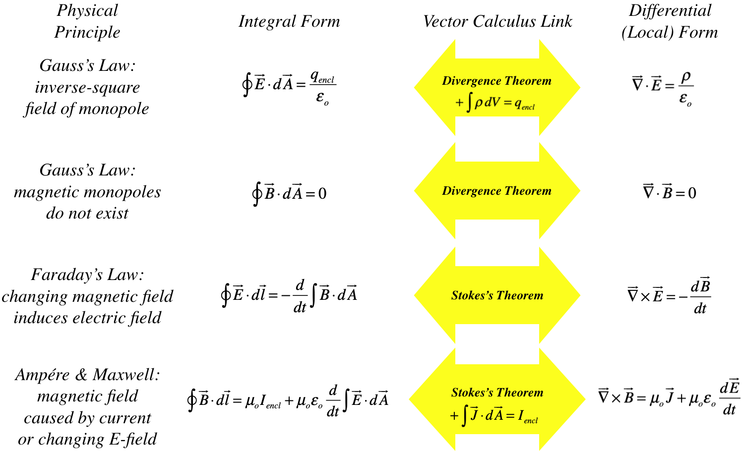
Let’s start at a place as good as any: simplifying Maxwell’s original equations. We’ll be focusing on the differential forms for this post, but for posterity here’s a brief recap of the whole set of equations and the physics they describe.

Credit: [Physics Libretexts]
Four differential equations to describe two fields is a lot no matter how symmetric those equations might be, so let’s see if we can perform some mathematical trickery to fix that.
Math Tricks
Looking at Faraday’s Law, for example, we know the curl of the electric field is equal to the negative time-derivative of the magnetic field: if we could write that RHS as the curl of some field as well we’d be able to cancel the operation from both sides.
One way you might think of getting this result would be to write, purely for mathematical convenience, the magnetic field as the curl of some other arbitrary vector field. This would allow us to switch the partial derivative and curl around to write the time-derivative of the magnetic field as the curl of the time-derivative of some other field we’ll call \( \textbf{A} \) as shown below:
\nabla \times \textbf{E}= -\frac{\partial \textbf{B}}{\partial t}= -\frac{\partial }{\partial t}(\nabla \times \textbf{A})\nabla \times \textbf{E}=-\nabla \times \frac{\partial \textbf{A}}{\partial t}This looks promising: we have a curl operator on both sides we can just cancel to get our electric field!
Degrees of Freedom
Unfortunately, the curl’s inverse isn’t that straightforward. Think about the relationship differentiation and integration have with the constant term of a function. The derivative of any constant is zero, thus when attempting to reconstruct the original function via integration we’re left with an unknown constant term at the end of our expression: as a result, without an extra piece of info such as an (x,y) pair the function has a degree of freedom left unspecified.
\int{f'(x)dx}=f(x)+C


Similarly, undoing the curl operation on both sides with some “anti-curl” operation leaves a term undefined: the curl of the gradient of any vector field is zero, thus instead of a constant, a whole gradient is left unspecified.
\nabla \times \nabla \psi=0
\nabla^{-1}\times(-\nabla \times \frac{\partial \textbf{A}}{\partial t})=-\frac{\partial \textbf{A}}{\partial t}+\nabla \psi \:\:\:\: (1)Luckily, we do have that extra piece of info to pull from another area of physics. We’ve used voltage all the time in electrostatics, and we know the electric field is defined here as the negative gradient of the electrostatic potential it comes from. This is reflected by the curl of the electric field being zero (this is what Kirchhoff’s Law states when it’s used for the conservation of voltage in circuit analysis!) in electrostatics: without a magnetic field the only term defining the electric field is a gradient, and the curl of a gradient is always zero.
Viewed as a coordinate relationship, the extra bit of info we have is that when no magnetic field is present—and hence \( A=0 \)—the electric field has the value \( E=-\nabla \varphi \), where \( \varphi \) is the electrostatic potential. Substituting that into (1) we find the following expression for our electric field:
(\textbf{A}, \textbf{E})\longrightarrow (0, -\nabla \varphi)\textbf{E}= -\frac{\partial \textbf{A}}{\partial t} - \nabla \varphi\:\:\:\:\:(2)Ok…that works, but we’ve done a lot of mathematical juggling that might seem disconcerting—not to mention we have this whole new magnetic field to deal with! In fact, our feeling of accomplishment with defining our arbitrary vector field as the electrostatic potential is equally hollow from a theoretical perspective: just because we’ve worked with \( \varphi \) before as a tool doesn’t make it any less arbitrary than \( \textbf{A} \) as far as Maxwell’s equations are concerned. If we treat Maxwell’s equations as the postulates of electromagnetism from which all other laws follow, then we now have two quantities to define on our hands.
Starting off, we can check that our definition of the magnetic field in terms of this new field \( \textbf{A} \) abides by Gauss’s Law for magnetic fields. Using similar logic as last time to undo the operation on both sides, canceling the dot product on both sides leaves an added degree of freedom in the form of a curl field. As shown below, this happens to work out to the exact same result we found with our last derivation: the magnetic field can be expressed as the curl of some arbitrary vector field \( \textbf{A} \).
\nabla \cdot \textbf{B}=0\nabla \cdot (\nabla \times \textbf{A})=0\textbf B=\nabla \times \textbf A \:\:\:\:(3)
It seems like our mathematical trickery of defining this new field \( \textbf A \) has worked out so far: although it’s more indirect, we’ve encapsulated Gauss’s Law of Magnetism and Faraday’s Law with the definitions of these vector and scalar fields!
Maxwell’s Equations in Potential Form
The method of introducing these fields we employed was pretty artificial, but that should illustrate an important point about how these fields were devised in the first place: they were defined post-hoc as mathematical tools that were constructed to conform to existing results like Faraday’s Law. At this point, it might seem like more trouble than it’s worth to work with these at all, but let’s give them a shot and see how they represent the rest of Maxwell’s equations. We’ve encapsulated Gauss’s Law for Magnetism and Faraday’s Law in our definitions of the electric and magnetic fields so that leaves two more laws to take care of:
Gauss's \:Law \:for \:Electricity:\: \nabla \cdot \textbf{E}=\frac{\rho}{\epsilon_0}Ampere-Maxwell\: Law:\:\nabla \times \textbf B=\mu_0\textbf j +\epsilon_0\mu_0\frac{\partial\textbf E}{\partial t}We can start by replacing each instance of \( \textbf E \) and \( \textbf B \) with their scalar and vector field counterparts and apply some basic identities to knock out extra terms. Here’s the work for Gauss’s Law (vector identities employed at each step are separated from the main equation by a colon and are written with the unused variable V)…
\nabla \cdot (-\frac{\partial \textbf{A}}{\partial t} - \nabla \varphi)=\frac{\rho}{\epsilon_0}:\:\nabla \cdot (\nabla V) =\nabla^2V\frac{\partial}{\partial t}(\nabla \cdot\textbf{A})+\nabla^2\varphi=-\frac{\rho}{\epsilon_0}\:\:\:\: (4)…and finally, the Ampere-Maxwell Law:
\nabla \times (\nabla \times \textbf{A})=\mu_0\textbf j+\epsilon_0\mu_0\frac{\partial}{\partial t}(-\frac{\partial \textbf{A}}{\partial t} - \nabla \varphi): \nabla \times (\nabla \times \textbf{V})=\nabla (\nabla \cdot \textbf V)-\nabla^2\textbf{V}\nabla (\nabla \cdot \textbf A)-\nabla^2\textbf{A}=\mu_0\textbf j-\epsilon_0\mu_0\frac{\partial^2\textbf{A}}{\partial t^2} - \nabla(\mu_0\epsilon_0 \frac{\partial \varphi}{\partial t})\nabla^2\textbf{A}-\epsilon_0\mu_0\frac{\partial^2\textbf{A}}{\partial t^2}-\nabla (\nabla \cdot \textbf A +\mu_0\epsilon_0 \frac{\partial \varphi}{\partial t})=-\mu_0\textbf j \:\:\;\: (5)These results aren’t bad at all: we’ve successfully translated our four first-order, symmetric differential equations for the electric and magnetic fields for two second-order, asymmetric differential equations for two new fields. But that asymmetry is off-putting for a system that’s supposed to simplify problems—not to mention that the subset of problems in classical E&M in which these new fields come in handy is limited anyway. Does that mean this whole exercise was a complete waste of time?
Gauge Fixing
\textbf{E}= -\frac{\partial \textbf{A}}{\partial t} - \nabla \varphi\:\:\:\:\:(2)\textbf B=\nabla \times \textbf A \:\:\:\:(3)
The two equations above are fundamental results, derived solely from Maxwell’s equations and two newly defined fields. But at this point you may be understandably disappointed with our results: after all, we’ve reduced our description of the electric and magnetic potentials to two equations, but none of them have much in the way of symmetry as our original equations did, and to actually get our real fields requires another layer of equations! What was the point of this whole exercise?
It’s at this point that we turn back to our prelude of number-juggling for guidance: we know that our electric and magnetic potentials are mathematical constructs, and because of that they have more degrees of freedom in the form of their divergence and curl than what’s specified by our electric and magnetic fields.
Here, we rely on that lack of restriction by turning our attention to the dot product of \( \textbf A \): because the dot product and cross product are completely independent, fixing the cross product so that we end up with a single magnetic field doesn’t prevent us from changing the dot product however we want. That leaves us to choose just what value’s most convenient to us!
\textbf{A}'=\textbf{A}+\nabla \psi\:\:\:\: (6)\textbf{B}'=\nabla \times (\textbf{A}+\nabla \psi)\nabla \times (\textbf{A}+\nabla \psi)=\nabla \times \textbf{A}=\textbf{B}The calculations above confirm the invariance we already know about \( \textbf{A} \), but to make sure our real fields are both unchanged we have to adjust the electric field too. To achieve this we can turn to our electrostatic potential: by making an appropriate adjustment to this scalar field, we can make sure any change to \( \textbf{A} \) is canceled out! Here’s the proof below:
\varphi'=\varphi-\frac{\partial \psi}{\partial t} \:\:\:\: (7)\textbf{E}'=-\frac{\partial}{\partial t}(\textbf{A}+\nabla \psi)-\nabla(\varphi-\frac{\partial \psi}{\partial t})-\frac{\partial}{\partial t}(\textbf{A}+\nabla \psi)-\nabla(\varphi-\frac{\partial \psi}{\partial t})=-\frac{\partial \textbf{A}}{\partial t}-\nabla(\varphi-\frac{\partial \psi}{\partial t}-\frac{\partial \psi}{\partial t})-\frac{\partial \textbf{A}}{\partial t}-\nabla(\varphi-\frac{\partial \psi}{\partial t}-\frac{\partial \psi}{\partial t})=-\frac{\partial \textbf{A}}{\partial t}-\nabla \varphi=\textbf{E}With our physics unchanged and our math made far more versatile, we can finally start to reap some of the benefits of this exercise. Let’s take a look!
The Coulomb Gauge
Right away, one choice might stand out based on our equations: why not just get rid of the terms entirely by setting \( \nabla \cdot \textbf {A}=0 \)? If we plug that into (4) and (5) and simplify our equations, we get the results below:
\nabla^2\varphi=-\frac{\rho}{\epsilon_0}\:\:\:\:(8)\nabla^2\textbf{A}-\epsilon_0\mu_0\frac{\partial^2\textbf{A}}{\partial t^2}-\mu_0\epsilon_0 \frac{\partial (\nabla\varphi)}{\partial t}=-\mu_0\textbf j \:\:\:\: (9)As far as partial differential equations go, these aren’t too bad— the electric potential equation especially is in a well-known form called the Poisson equation. Unfortunately, the magnetic potential doesn’t have an explicit solution and is much more hairy to work with, and since the electric field involves the time derivative of the magnetic potential in its definition that handicaps its use.
Luckily, there are many useful problems where this isn’t an issue: problems with constant magnetic fields generated by steady currents, for instance, will have \( \frac{\partial A}{\partial t}=0 \) where the electric field is solely determined by the electrostatic potential. That lets us set the second time derivative of \( A \) and the electric potential to zero (steady flow of currents implies constant potential difference driving that flow).
\nabla^2\varphi=-\frac{\rho}{\epsilon_0}\:\:\:\:\:\:(10)\nabla^2\textbf{A}=-\mu_0\textbf j\:\:\:\:(11)This leaves us with two symmetric and independent Poisson equations, and this makes solving much easier: in fact, going through the grunge work of solving these differential equations (for more on solving these kinds of PDEs, look up Green’s Functions) gives us two familiar laws:
\varphi(r)=\frac{1}{4\pi\epsilon_0}\int_{V'}\frac{{\rho(\textbf{r'})}}{|\textbf{r}-\textbf{r'}|}d^3r'\:\:\:\:(12)\textbf{A}(r)=\frac{\mu_0}{4\pi}\int_{V'}\frac{\textbf{j(r')}}{|\textbf{r}-\textbf{r'}|}d^3r'\:\:\:\:\:\:\:\:(13)The first equation is our standard electrostatic potential from which we can derive Coulomb’s Law, but the bottom equation should be familiar as well: its symmetry with the electrostatic potential is beautiful, of course—it’s where it gets its name as the “magnetic vector potential”—but it’s also just one step removed from the magnetostatic analog of Coulomb’s Law: the Biot Savart law for steady currents.

Credit: [Physics Libretexts]
If you weren’t sold on the practicality of these equations before then hopefully the added power of gauge fixing convinces you: we’ve managed to analytically derive two extremely important laws in electrostatics and magnetostatics, and all thanks to two fake fields and an added layer of arbitrary assumptions! This method of choosing the most convenient value of a field for the problem at hand is called “gauge fixing,” and theories that employ it are called “gauge theories.” Classical electrodynamics was the first, but, as we’ll soon get a taste of, gauge theories have come to dominate modern physics today.
The Causality Problem

Credit: [Wikimedia Commons]
The gauge we just employed is called the Coulomb Gauge, and these kinds of special cases are where it shines. What’s most amazing about gauge theories is that these arbitrarily chosen equations are still valid across physics. One of the most common misunderstandings around the Coulomb-gauged electric potential is that it violates special relativity: a consequence of relativity is that observed changes to a physical system can’t propagate faster than lightspeed, but since the Poisson equation doesn’t have any terms that change with time it seems like any change to the field’s source charges can affect space lightyears away instantly. If that’s the case, how can these fields still be real?
The answer is, no, they can’t be real. Or more specifically, they can’t be measurable. Although special relativity prevents information from instantly traveling across distances, for a field to carry information it has to be observable through some kind of physical measurement, and since these fields don’t have a direct physical meaning in classical electromagnetism they manage to skirt this rule. Relativity effectively gives us a way to put the physical nature of a field to the test: although the values of the unmeasurable potentials can contribute to measurable changes in the electric and magnetic fields (those changes take time to propagate), instant changes to the potential field itself don’t have the same effect.
The Lorenz (NOT “Lorentz”) Gauge
The math behind separating the instantaneous change of the vector potential and the delayed change of its resultant physical fields is messy, but through such proofs, we can show that any gauge transformation preserves all laws of electromagnetism—that leaves the choice of which one we use for a given problem entirely up to us. In the case of the Coulomb Gauge, its asymmetric form makes them less than ideal for many other cases where the electric and magnetic fields are both changing, so we look to our original equations and pick out another value for \( \textbf{A} \) that cancels the electric potential from the second equation entirely. Setting \( \textbf{A}=-\epsilon_0\mu_0\frac{\partial \varphi}{\partial t} \) we find the following set of equations below:
\nabla^2\varphi-\epsilon_0\mu_0\frac{\partial^2\varphi}{\partial t^2}=-\frac{\rho}{\epsilon_0}\:\:\:\: (14)\nabla^2\textbf{A}-\epsilon_0\mu_0\frac{\partial^2\textbf{A}}{\partial t^2}=-\mu_0\textbf j \:\:\;\: (15)The D’Alembertian Operator
We mentioned before how the Coulomb Gauge is messy to work with in areas like special relativity. Thankfully, this choice of gauge transformation happens to resolve this, and so physicists represent this harmony by writing the equations in terms of the D’Alembertian, an operator with nice properties in special relativity, to rewrite the electromagnetic fields in a way convenient for problem-solving (the operator is a generalization of the Laplacian to time-dependent systems, and with some background in special relativity we can tell from the form that the operator is invariant under Lorentz transformations, which form the isometry group of Minkowski space).
\Box^2\equiv\nabla^2-\frac{1}{c^2}\frac{\partial^2}{\partial t^2}If you’re wondering where we’ll insert the \( \frac{1}{c^2} \) into our electromagnetic equations, recall that the speed of light is defined as \( c^2=\frac{1}{\epsilon_0\mu_0} \), and thus we already have \( \frac{1}{c^2}=\epsilon_0\mu_0 \) represented in our current equations. Written below, we get our final set of equations under what is called the Lorenz Gauge—NOT to be confused with Lorentz transformations, which is an operation under which this gauge is commonly used and thus is misnamed often in many sources—and represents a more generally applicable form in which we work with electromagnetic fields.
\Box^2\varphi=-\frac{\rho}{\epsilon_0}\:\:\:\: (16)\Box^2\textbf{A}=-\mu_0\textbf{j}\:\:\:\: (17)There are obviously other gauge transformations possible for the potential fields, but these are the two most commonly used in physics and engineering. And ultimately, that’s what the point of these potentials is in classical and relativistic mechanics: they’re mathematical constructs with an intangible nature that makes them easy to mold into whatever equations suit a problem best, but ultimately aren’t real fields like the electric and magnetic fields they represent.
…right?
Fine…We’ll Talk About Quantum Mechanics
If you’re familiar with the mind-bending probabilities and uncertainties of quantum mechanics, it might not be a surprise to learn that E&M in the world of quantum electrodynamics, or QED, is a bit of a paradigm shift from its classical counterpart. Because describing full proofs for the next couple of results would require an entire crash course on modern physics, we’re gonna have to take scientists like Richard Feynman for their word when given a particular formula and focus on the implications of QED’s upside-down results in relation to our familiar fields.
First things first…the potentials matter more than the fields they describe. In quantum mechanics, the position and momentum of a particle aren’t fixed at single values but instead a spread of possible states defined by a wave-like distribution called a wave function. Describing how the properties of this wave— where notions such as momentum can be determined from the amplitude and wavelength—vary in space and time, as well as how these wave particles interact and interfere with one another is key to any subatomic model of physics.

Credit: [The Scientific Gamer]
In the famous double-slit experiment, for example, the position a particle strikes the wall F after being fired from point A depends on the way its wave function travels through space, splitting into two waves at the two slits S2 that can interfere with each other based on the way their peaks align. The peaks of a wave shift position based on its phase, which makes the phase difference between waves B and C (the waves generated from slit B and slit C respectively) important for when these two waves hit the wall, where the areas enriched by both waves are areas where the particle is most likely to appear and those where the waves canceled each other out are the least.
Potentials and Phase Difference
It just so happens that our vector potentials are ideal for describing this phase difference: assuming (for simplicity’s sake) waves B and C start at the same phase at their respective slits, the difference between them is based on how the waves change over their trajectory to the wall, and when these trajectories pass through electric and magnetic fields their phase change is given by the following pair of equations. This phase manifests in several places, but to analyze our double-slit experiment, the phase difference between the two waves manifests in a shifted position of the interference pattern on wall F.
\Delta\Phi_{\textbf{E}}=\frac{q}{\hbar}\int \varphi\: dt \:\:\:\: (18)\Delta\Phi_{\textbf{B}}=\frac{q}{\hbar}\int_{\textbf{Path}}\textbf{A}\cdot d\textbf{l}\:\:\:\: (19)But this isn’t just a one-off place where the potentials take precedence over the force fields: for various reasons, it’s much easier to describe quantum interactions between particles in terms of energy and momentum instead of forces, which means that the potentials end up taking on a much more important role for describing physical phenomenon altogether than the force fields they produce.
Still, though, by using our original definition of \( B \) in terms of \( A \) and \( E \) in terms of [/latex] \varphi [/latex] we can still technically rewrite these laws in terms of our physical fields. So there’s still nothing real about these potentials, right?
The Aharonov-Bohm Effect
Unfortunately, there are cases in quantum mechanics where this line becomes fundamentally blurred. Imagine a long solenoid, a spring-like coil of wire where each loop generates its own magnetic field in response to a changing electric current passing through it: the fields on the outside cancel out and approach zero as the solenoid grows arbitrarily long, and add up on the inside, producing a situation where only the inside of the loop contains a magnetic field.

Credit: [TikZ Graphics]
But remember, the fact that \( B \) is fixed at 0 outside the solenoid tells us nothing about \( A \): since our magnetic field lines are practically horizontal through the solenoid, we can imagine the vector potential lines as forming circular paths around the coil.
Now let’s imagine our double-slit experiment repeated, but where waves B and C pass through the region outside a solenoid. Sure enough, they pass through \( A \) and the resulting distribution of particle positions on wall F will experience the predicted wave shift: in other words, we’ve demonstrated a case where the vector potential, not the magnetic field, creates a change in the wave function, and correspondingly the distribution of positions a particle will assume!
This clever trick that first revealed the vector potential’s influence—known after its co-discoverers as the Aharonov-Bohm effect—was discovered nearly thirty years after this formulation of quantum mechanics was created. Of course, the methods used to demonstrate its nature are ingenious, but I also think its ability to hide in plain sight for so long also reveals the power of the hidden assumptions we make about physics, and what we deem is and isn’t “real.”
The simulation below (available at the Wolfram Demonstrations Project) displays this phenomenon in practice: adjusting the solenoid’s magnetic field applies a phase shift to the interference pattern on the wall as described.
Remember, the entire idea of fields is to provide a framework for thinking about “action at a distance.” Even if a magnetic field is present, the fact that it has a value of zero at all points along the particle’s path means that it can’t have any effect on the particle, and thus the courier of action must be the vector potential as the only remaining field: in quantum mechanics, the vector potential is more real than the classical magnetic field!
Gauge Invariance in QED
One last thing. This whole business of determining the phase shift of a wave function from the vector potential begs the question of whether we can do the converse: do we finally have a way to pin down the physical value of our potentials? Let’s try applying a valid gauge transformation to our vector potential and see how it affects the phase shift integral:
\oint_{\textbf{Path}}\textbf{A}'\cdot d\textbf{s}= \oint_{\textbf{Path}}(\textbf{A}+\nabla\psi)\cdot d\textbf{l}If we separate terms and apply Stokes’s Theorem to the second integral we can immediately see the dreaded identity creep up again: the closed line integral of a conservative vector field is always zero, and that means our potential still has that same gradient of freedom.
\oint_{\textbf{Path}}(\textbf{A}+\nabla\psi)\cdot d\textbf{l}=\oint_{\textbf{Path}}\textbf{A}\cdot d\textbf{l}\:+\oint_{\textbf{Path}}\nabla\psi\cdot d\textbf{l}\oint_{\textbf{Path}}\nabla\psi\cdot d\textbf{l}=\iint(\nabla\times[\nabla \psi])\cdot d\textbf{S}=0\oint_{\textbf{Path}}(\textbf{A}+\nabla\psi)\cdot d\textbf{l}=\oint_{\textbf{Path}}\textbf{A}\cdot d\textbf{s}Our field achieves the feat of being physically “real” but still indeterminate! Unfortunately, we still have to rely on gauge fixing to fix our physics.
Conclusion
So…what exactly are these potentials? We’ve covered their derivation and representation with Maxwell’s equations and the ways their gauge symmetry can be manipulated to derive the Biot-Savart law with one choice and solve problems in relativistic physics with the other. And thanks to quantum mechanics, we’ve even gotten a glimpse into the far-reaching implications of these potentials thanks to phenomena like the Aharonov-Bohm effect. But that search has led us to treat these fields as anything from mathematical shortcuts in a certain subset of problems to physical entities with observable effects on the world: which one is it?
The answer, as dissatisfying as it sounds, is that it doesn’t matter—at least, as far as physics is concerned. What values in an equation we deem to be “real” is a question that cuts to the heart of realist vs. idealist scientific philosophy, but isn’t a question that has a factual answer. If you define a “real field” as causing a physical change to the region it extends, then sure, the vector potential is “real”… but if you make the reasonable objection that something “real” should have a single value instead of leaving it open-ended, then it’s not “real.” As far as the pragmatic physicist is concerned, it’s best to abide by the even more fundamental maxim of scientific philosophy: if it works, it works.
What’s Next?
But although the question of whether a gauge-invariant quantity is “real” might be a philosophical one, other aspects of gauge symmetry aren’t, and they can give us a more wide-ranging lens to view electromagnetism and other gauge theories like it—all the way up to the current Standard Model of Physics. For example, if choosing a gauge is like choosing a coordinate system, then what are the properties of this coordinate system? If gauge freedoms stem from changes that leave some quantity invariant, then what is that quantity, and what determines the type of gauge transformation that leaves it that way?
These aren’t questions about physics or philosophy—instead, they’re about math. And these are the questions we’ll be tackling in the next post: in what’ll start as a crash course in Lagrangian mechanics, a detour into group theory will help us zoom out from electromagnetic potentials to the full reaches of gauge theories and the math that ties together physics today. See you then!